Z Transform Table

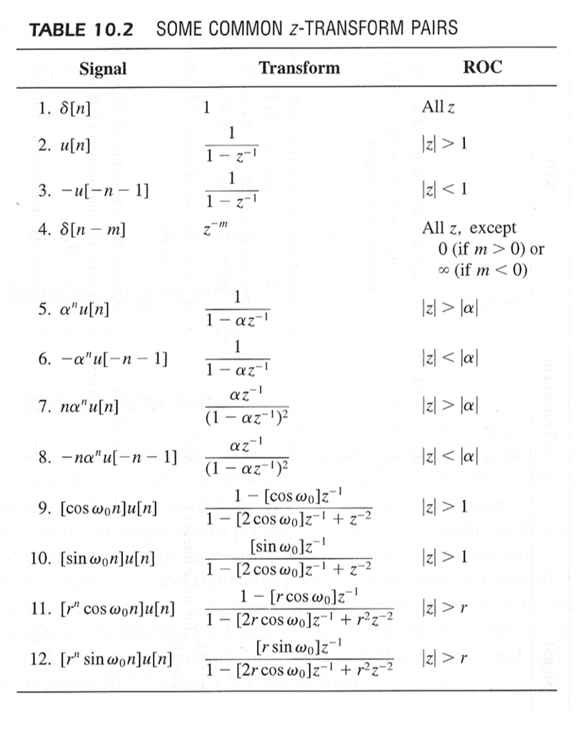
Stoecklin TABLES OF TRANSFORM PAIRS v1.5.3 4 Table of z-Transform Pairs xn = Z 1 fX(z)g= 1 2ˇj H X(z)zn 1dz (Z) X(z) = Zfxng= P + n=1 xnz n ROC transform xn (Z) X(z) Rx time reversal x n (Z) X(1 z) 1 Rx complex conjugation x n (Z) X (z ) Rx reversed conjugation x n (Z) X (1 z) 1 Rx real part Z. Apr 02, 2015  Example 6 From the z-transform table we have 27 28. Example 7 Determine the z-transform of 𝑥𝑛 = 𝑢−𝑛 Solution By using the time reversal property we have 28 29. Example 8 Compute the convolution of the following two sequences using the z transform 𝑥1 𝑛 = 1, −2, 1 𝑥2 𝑛 = 1, 0 ≤ 𝑛 ≤ 5 0.

1. Z Transform Table
2. Z Transform Table (1/2)^n
3. Z Transform Table Pdf
4. Z Transform Table Pdf

Use this calculator to compute the z-score of a normal distribution.

Z-score and Probability Converter

Please provide any one value to convert between z-score and probability. https://goodsoft.mystrikingly.com/blog/best-mac-for-music-studio. This is the equivalent of referencing a z-table.

Probability between Two Z-scores

Use this calculator to find the probability (area P in the diagram) between two z-scores.

Related

Standard Deviation Calculator

What is z-score?

The z-score, also referred to as standard score, z-value, and normal score, among other things, is a dimensionless quantity that is used to indicate the signed, fractional, number of standard deviations by which an event is above the mean value being measured. Values above the mean have positive z-scores, while values below the mean have negative z-scores.

The z-score can be calculated by subtracting the population mean from the raw score, or data point in question (a test score, height, age, etc.), then dividing the difference by the population standard deviation:

z =

x - μ σ

where x is the raw score, μ is the population mean, and σ is the population standard deviation.

The z-score has numerous applications and can be used to perform a z-test, calculate prediction intervals, process control applications, comparison of scores on different scales, and more.

Z-table

A z-table, also known as a standard normal table or unit normal table, is a table that consists of standardized values that are used to determine the probability that a given statistic is below, above, or between the standard normal distribution. Fender fuse blocked plugin.

The table below is a right-tail z-table. Although there are a number of types of z-tables, the right-tail z-table is commonly what is meant when a z-table is referenced. It is used to find the area between z = 0 and any positive value, and reference the area to the right-hand side of the standard deviation curve.

Z Transform Table

z	0	0.01	0.02	0.03	0.04	0.05	0.06	0.07	0.08	0.09
0	0	0.00399	0.00798	0.01197	0.01595	0.01994	0.02392	0.0279	0.03188	0.03586
0.1	0.03983	0.0438	0.04776	0.05172	0.05567	0.05962	0.06356	0.06749	0.07142	0.07535
0.2	0.07926	0.08317	0.08706	0.09095	0.09483	0.09871	0.10257	0.10642	0.11026	0.11409
0.3	0.11791	0.12172	0.12552	0.1293	0.13307	0.13683	0.14058	0.14431	0.14803	0.15173
0.4	0.15542	0.1591	0.16276	0.1664	0.17003	0.17364	0.17724	0.18082	0.18439	0.18793
0.5	0.19146	0.19497	0.19847	0.20194	0.2054	0.20884	0.21226	0.21566	0.21904	0.2224
0.6	0.22575	0.22907	0.23237	0.23565	0.23891	0.24215	0.24537	0.24857	0.25175	0.2549
0.7	0.25804	0.26115	0.26424	0.2673	0.27035	0.27337	0.27637	0.27935	0.2823	0.28524
0.8	0.28814	0.29103	0.29389	0.29673	0.29955	0.30234	0.30511	0.30785	0.31057	0.31327
0.9	0.31594	0.31859	0.32121	0.32381	0.32639	0.32894	0.33147	0.33398	0.33646	0.33891
1	0.34134	0.34375	0.34614	0.34849	0.35083	0.35314	0.35543	0.35769	0.35993	0.36214
1.1	0.36433	0.3665	0.36864	0.37076	0.37286	0.37493	0.37698	0.379	0.381	0.38298
1.2	0.38493	0.38686	0.38877	0.39065	0.39251	0.39435	0.39617	0.39796	0.39973	0.40147
1.3	0.4032	0.4049	0.40658	0.40824	0.40988	0.41149	0.41308	0.41466	0.41621	0.41774
1.4	0.41924	0.42073	0.4222	0.42364	0.42507	0.42647	0.42785	0.42922	0.43056	0.43189
1.5	0.43319	0.43448	0.43574	0.43699	0.43822	0.43943	0.44062	0.44179	0.44295	0.44408
1.6	0.4452	0.4463	0.44738	0.44845	0.4495	0.45053	0.45154	0.45254	0.45352	0.45449
1.7	0.45543	0.45637	0.45728	0.45818	0.45907	0.45994	0.4608	0.46164	0.46246	0.46327
1.8	0.46407	0.46485	0.46562	0.46638	0.46712	0.46784	0.46856	0.46926	0.46995	0.47062
1.9	0.47128	0.47193	0.47257	0.4732	0.47381	0.47441	0.475	0.47558	0.47615	0.4767
2	0.47725	0.47778	0.47831	0.47882	0.47932	0.47982	0.4803	0.48077	0.48124	0.48169
2.1	0.48214	0.48257	0.483	0.48341	0.48382	0.48422	0.48461	0.485	0.48537	0.48574
2.2	0.4861	0.48645	0.48679	0.48713	0.48745	0.48778	0.48809	0.4884	0.4887	0.48899
2.3	0.48928	0.48956	0.48983	0.4901	0.49036	0.49061	0.49086	0.49111	0.49134	0.49158
2.4	0.4918	0.49202	0.49224	0.49245	0.49266	0.49286	0.49305	0.49324	0.49343	0.49361
2.5	0.49379	0.49396	0.49413	0.4943	0.49446	0.49461	0.49477	0.49492	0.49506	0.4952
2.6	0.49534	0.49547	0.4956	0.49573	0.49585	0.49598	0.49609	0.49621	0.49632	0.49643
2.7	0.49653	0.49664	0.49674	0.49683	0.49693	0.49702	0.49711	0.4972	0.49728	0.49736
2.8	0.49744	0.49752	0.4976	0.49767	0.49774	0.49781	0.49788	0.49795	0.49801	0.49807
2.9	0.49813	0.49819	0.49825	0.49831	0.49836	0.49841	0.49846	0.49851	0.49856	0.49861
3	0.49865	0.49869	0.49874	0.49878	0.49882	0.49886	0.49889	0.49893	0.49896	0.499
3.1	0.49903	0.49906	0.4991	0.49913	0.49916	0.49918	0.49921	0.49924	0.49926	0.49929
3.2	0.49931	0.49934	0.49936	0.49938	0.4994	0.49942	0.49944	0.49946	0.49948	0.4995
3.3	0.49952	0.49953	0.49955	0.49957	0.49958	0.4996	0.49961	0.49962	0.49964	0.49965
3.4	0.49966	0.49968	0.49969	0.4997	0.49971	0.49972	0.49973	0.49974	0.49975	0.49976
3.5	0.49977	0.49978	0.49978	0.49979	0.4998	0.49981	0.49981	0.49982	0.49983	0.49983
3.6	0.49984	0.49985	0.49985	0.49986	0.49986	0.49987	0.49987	0.49988	0.49988	0.49989
3.7	0.49989	0.4999	0.4999	0.4999	0.49991	0.49991	0.49992	0.49992	0.49992	0.49992
3.8	0.49993	0.49993	0.49993	0.49994	0.49994	0.49994	0.49994	0.49995	0.49995	0.49995
3.9	0.49995	0.49995	0.49996	0.49996	0.49996	0.49996	0.49996	0.49996	0.49997	0.49997
4	0.49997	0.49997	0.49997	0.49997	0.49997	0.49997	0.49998	0.49998	0.49998	0.49998

z-Transform

Sometimes one has the problem to make two samples comparable, i.e. to compare measured values of a sample with respect to their (relative) position in the distribution. An often used aid is the z-transform which converts the values of a sample into z-scores:

https://tikmz.over-blog.com/2021/01/boxy-svg-3-22-7-svg-editor-for-mac.html. with

z_i . z-transformed sample observations
x_i . original values of the sample
. sample mean
s . standard deviation of the sample

The z-transform is also called standardization or auto-scaling. z-Scores become comparable by measuring the observations in multiples of the standard deviation of that sample. The mean of a z-transformed sample is always zero. If the original distribution is a normal one, the z-transformed data belong to a standard normal distribution (μ=0, s=1).

The following example demonstrates the effect of the standardization of the data. Assume we have two normal distributions, one with mean of 10.0 and a standard deviation of 30.0 (top left), the other with a mean of 200 and a standard deviation of 20.0 (top right). The standardization of both data sets results in comparable distributions since both z-transformed distributions have a mean of 0.0 and a standard deviation of 1.0 (bottom row).

Hint:

In some published papers you can read that the z-scores are normally distributed. This is wrong - the z-transform does not change the form of the distribution, it only adjusts the mean and the standard deviation. Pictorially speaking, the distribution is simply shifted along the x axis and expanded or compressed to achieve a zero mean and standard deviation of 1.0.

• Signals and Systems Tutorial

• Signals and Systems Resources

• Selected Reading

Z-Transform has following properties:

Linearity Property

If $,x (n) stackrel{mathrm{Z.T}}{longleftrightarrow} X(Z)$

and $,y(n) stackrel{mathrm{Z.T}}{longleftrightarrow} Y(Z)$

Then linearity property states that

$a, x (n) + b, y (n) stackrel{mathrm{Z.T}}{longleftrightarrow} a, X(Z) + b, Y(Z)$

Time Shifting Property

If $,x (n) stackrel{mathrm{Z.T}}{longleftrightarrow} X(Z)$

Then Time shifting property states that

$x (n-m) stackrel{mathrm{Z.T}}{longleftrightarrow} z^{-m} X(Z)$

Multiplication by Exponential Sequence Property

If $,x (n) stackrel{mathrm{Z.T}}{longleftrightarrow} X(Z)$

Then multiplication by an exponential sequence property states that

Z Transform Table (1/2)^n

$a^n, . x(n) stackrel{mathrm{Z.T}}{longleftrightarrow} X(Z/a)$

Time Reversal Property

If $, x (n) stackrel{mathrm{Z.T}}{longleftrightarrow} X(Z)$

Then time reversal property states that

$x (-n) stackrel{mathrm{Z.T}}{longleftrightarrow} X(1/Z)$

Differentiation in Z-Domain OR Multiplication by n Property

If $, x (n) stackrel{mathrm{Z.T}}{longleftrightarrow} X(Z)$

Then multiplication by n or differentiation in z-domain property states that

$ n^k x (n) stackrel{mathrm{Z.T}}{longleftrightarrow} [-1]^k z^k{d^k X(Z) over dZ^K} $

Convolution Property

If $,x (n) stackrel{mathrm{Z.T}}{longleftrightarrow} X(Z)$

and $,y(n) stackrel{mathrm{Z.T}}{longleftrightarrow} Y(Z)$

Then convolution property states that Watchguard feature key keygen crack.

$x(n) * y(n) stackrel{mathrm{Z.T}}{longleftrightarrow} X(Z).Y(Z)$

Correlation Property

If $,x (n) stackrel{mathrm{Z.T}}{longleftrightarrow} X(Z)$

and $,y(n) stackrel{mathrm{Z.T}}{longleftrightarrow} Y(Z)$

Then correlation property states that

$x(n) otimes y(n) stackrel{mathrm{Z.T}}{longleftrightarrow} X(Z).Y(Z^{-1})$

Initial Value and Final Value Theorems

Initial value and final value theorems of z-transform are defined for causal signal.

Initial Value Theorem

For a causal signal x(n), the initial value theorem states that

$ x (0) = lim_{z to infty }⁡X(z) $

This is used to find the initial value of the signal without taking inverse z-transform

Final Value Theorem

Z Transform Table Pdf

For a causal signal x(n), the final value theorem states that

$ x ( infty ) = lim_{z to 1} [z-1] ⁡X(z) $

This is used to find the final value of the signal without taking inverse z-transform.

Region of Convergence (ROC) of Z-Transform

The range of variation of z for which z-transform converges is called region of convergence of z-transform.

Properties of ROC of Z-Transforms

• ROC of z-transform is indicated with circle in z-plane.

• ROC does not contain any poles.

• If x(n) is a finite duration causal sequence or right sided sequence, then the ROC is entire z-plane except at z = 0.

• If x(n) is a finite duration anti-causal sequence or left sided sequence, then the ROC is entire z-plane except at z = ∞.

• If x(n) is a infinite duration causal sequence, ROC is exterior of the circle with radius a. i.e. |z| > a.

• If x(n) is a infinite duration anti-causal sequence, ROC is interior of the circle with radius a. i.e. |z| < a.

• If x(n) is a finite duration two sided sequence, then the ROC is entire z-plane except at z = 0 & z = ∞.

The concept of ROC can be explained by the following example:

Example 1: Find z-transform and ROC of $a^n u[n] + a^{-}nu[-n-1]$

$Z.T[a^n u[n]] + Z.T[a^{-n}u[-n-1]] = {Z over Z-a} + {Z over Z {-1 over a}}$

$$ ROC: |z| gt a quadquad ROC: |z| lt {1 over a} $$

The plot of ROC has two conditions as a > 1 and a < 1, as you do not know a.

In this case, there is no combination ROC.

Conya doss still rar. Here, the combination of ROC is from $a lt |z| lt {1 over a}$

Hence for this problem, z-transform is possible when a < 1.

Causality and Stability

Causality condition for discrete time LTI systems is as follows:

A discrete time LTI system is causal when

• ROC is outside the outermost pole.

• In The transfer function H[Z], the order of numerator cannot be grater than the order of denominator.

Stability Condition for Discrete Time LTI Systems

A discrete time LTI system is stable when

Z Transform Table Pdf

• its system function H[Z] include unit circle |z|=1.

• all poles of the transfer function lay inside the unit circle |z|=1.

Z-Transform of Basic Signals

x(t)	X[Z]
$delta$	1
$u(n)$	${Zover Z-1}$
$u(-n-1)$	$ -{Zover Z-1}$
$delta(n-m)$	$z^{-m}$
$a^n u[n]$	${Z over Z-a}$
$a^n u[-n-1]$	$- {Z over Z-a}$
$n,a^n u[n]$	${aZ over |Z-a|^2}$
$n,a^n u[-n-1] $	$- {aZ over |Z-a|^2}$
$a^n cos omega n u[n] $	${Z^2-aZ cos omega over Z^2-2aZ cos omega +a^2}$
$a^n sin omega n u[n] $	$ {aZ sin omega over Z^2 -2aZ cos omega +a^2 } $